
This lesson explores algorithms and how repeated, carefully sized steps can improve a model’s predictions.
The Sandwich Robot
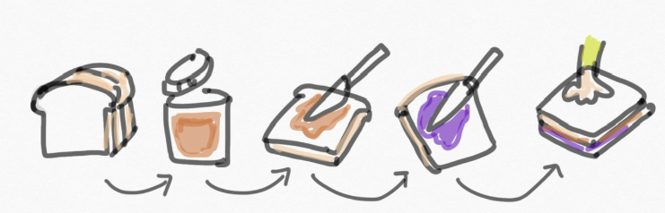
Imagine you’re programming a robot to make a peanut butter and jelly sandwich.
You say, “Make me a sandwich!” and the robot just stares at the counter.
You try again: “Put peanut butter on the bread!”
It grabs the jar and smears it on the outside of the bag.
You realize you need to give clear, step-by-step instructions:
- Pick up the bread.
- Open the peanut butter jar.
- Use a knife to spread peanut butter on one slice.
- Repeat with jelly on the other.
- Press slices together.
This is clearer. Can your partner find a step we still forgot, such as opening the bread bag or the jelly jar? You have started an algorithm — a recipe for solving a problem. Testing it helps us find missing instructions.
What Is an Algorithm?
An algorithm is a specific set of steps used to get something done.
We use them all the time, even without realizing it:
- Tying your shoes
- Solving a math problem
- Getting ready for school in the morning
Each one has an order and a purpose.
Computers do the same thing — they just follow algorithms written in code.
Try It Yourself — Write Your Own Algorithm
Pick something simple, like packing a school bag, arranging cards, or turning on a game console.
Write the steps in exact order, as if you were explaining it to a robot that doesn’t know anything.
Be specific. For example, to pack a notebook in a bag:
- Place the bag on a table with its opening facing up.
- Unzip the main compartment.
- Place the notebook inside the main compartment.
- Close the zipper.
Have a friend “follow” your algorithm exactly as written.
Did it work? If not, what went wrong?
That’s called debugging — fixing mistakes in your instructions.
Thinking Like a Data Scientist
Machine learning models depend on algorithms.
In one common approach to supervised learning, training repeats these steps:
- Look at data.
- Compare predictions to correct answers.
- Adjust the model’s parameters to try to reduce its error score.
That repeating process is a training algorithm. Its instructions can stay fixed while the model’s parameters change.
Gradient Descent — Improving One Step at a Time
In Lesson 8, our vending-machine observations were (2, 5), (3, 8), (4, 9), and (5, 10). We scored a line by its mean squared error (MSE): square each difference between observation and prediction, then average the squares.
For now, keep the slope at 2 and adjust just one knob, b, in prediction = 2 × input + b. Changing b shifts every prediction up or down.
Imagine a landscape where your position is a choice of b and your height is the error score. Gradient descent calculates the local slope of this error landscape and takes a step downhill. The learning rate controls the size of the update. A very small learning rate can make progress slow; a very large one can overshoot and increase the error.
The slope of this error landscape is different from the slope 2 in our prediction line. One tells us how error changes when b changes; the other tells us how predicted output changes when input changes.
Try It — Adjust One Knob
Start with b = 0. For this particular activity, repeat these instructions:
- Predict all four outputs using 2x + b.
- Subtract each prediction from its observed output to find the residual.
- Find the average residual.
- Add half the average residual to b.
- Calculate the new MSE. Repeat for three rounds.
First round: the predictions are 4, 6, 8, 10. The residuals are 1, 2, 1, 0. Their average is 1; half is 0.5. So b changes from 0 to 0.5. The new predictions are 4.5, 6.5, 8.5, 10.5.
Your turn: calculate the next value of b and its MSE before revealing the table. A calculator is welcome.
Check the next rounds
| Round | b | MSE |
|---|---|---|
| Start | 0 | 1.5 |
| 1 | 0.5 | 0.75 |
| 2 | 0.75 | 0.5625 |
| 3 | 0.875 | 0.515625 |
After round 1, the residuals are 0.5, 1.5, 0.5, −0.5. Their average is 0.5. Adding half of that to b = 0.5 gives b = 0.75.
Why not zero error? With slope fixed at 2, these noisy points cannot all lie on the same line. The best intercept is b = 1, where MSE = 0.5. Allowing the slope to change too can give a different, better-fitting line.
The half-sized update is a choice for this exercise, not a universal training rule. Here we stop after three rounds; training can also stop when changes in loss become very small or a set iteration limit is reached.
What If the Step Is Too Big?
Start again at b = 0. This time, add three times the average residual instead of half. The new b is 3. Work out the predictions and error score: did the bigger step help?
Reveal the oversized-step result
The predictions become 7, 9, 11, 13. Squared residuals are 4, 1, 4, 9, so MSE = 18 ÷ 4 = 4.5. The error rose from 1.5 to 4.5. A bigger update is not always better.
How This Connects to Machine Learning
In machine learning, algorithms are like the brain’s workout routine.
They decide how the computer learns patterns from data.
For example:
- A sorting algorithm can organize data when a task needs it; sorting is not a requirement for all training.
- An optimization algorithm, like gradient descent, adjusts parameters to reduce a chosen training loss.
- A clustering algorithm groups similar data points together without needing a correct output label for each example.
Each algorithm gives the computer a clear plan to reach its goal.
Takeaway Message
Algorithms are step-by-step guides for solving problems.
A training algorithm gives the instructions; the model’s parameters change. Lower training error is useful, but we must still test predictions on examples not used during training.
Optional Extensions
- Write a step-by-step algorithm for a task your class or family does every day — like making a smoothie or packing a bag. Then try to reduce the work it performs without changing the result. Count the operations: fewer written instructions do not always mean less work.
- Older students can explore simple coding challenges online that show how sorting, searching, and decision-making algorithms work in real life.
Optional Challenge — Compare Sorting Algorithms
Some problems take too long to solve by guessing or trial and error.
Different algorithms can take different amounts of work.
Think about sorting a deck of cards. You could:
- Find the smallest remaining card and put it at the next unfilled position. Repeat until all positions are filled (selection sort).
- Compare neighboring cards and swap them if they are out of order. Repeat passes through the cards until a full pass makes no swaps (bubble sort).
Both work, but one might take fewer steps.
Try each method on the same shuffled cards. Count comparisons and swaps separately; one pass is not always enough.
For older learners — the math behind our update
With slope fixed at 2, this dataset has MSE(b) = (b − 1)² + 0.5. The derivative is 2(b − 1). Adding half the average residual is exactly gradient descent on this MSE with learning rate 0.25. The main activity only requires arithmetic; calculus explains why the update points downhill.
